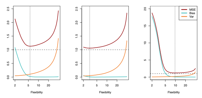
In all three cases, the variance increases and the bias decreases as the method’s flexibility increases. However, the flexibility level corresponding to the optimal test MSE differs considerably among the three data sets, because the squared bias and variance change at different rates in each of the data sets. 

In the left-hand panel of Figure, the bias initially decreases rapidly, resulting in an initial sharp decrease in the expected test MSE. 

On the other hand, in the center panel of Figure, the true f is close to linear, so there is only a small decrease in bias as flexibility increases, and the test MSE only declines slightly before increasing rapidly as the variance increases.

Finally, in the right-hand panel of Figure, as flexibility increases, there is a dramatic decline in bias because the true f is very non-linear. There is also very little increase in variance as flexibility increases. 

Consequently, the test MSE declines substantially before experiencing a small increase as model flexibility increases.

The relationship between bias, variance, and test set MSE is referred to as the bias-variance trade-off

Good test set performance of a statistical learning method re- quires low variance as well as low squared bias. This is referred to as a trade-off because it is easy to obtain a method with extremely low bias but high variance (for instance, by drawing a curve that passes through every single training observation) or a method with very low variance but high bias (by fitting a horizontal line to the data).

The challenge lies in finding a method for which both the variance and the squared bias are low.

What test set MSE actually measures

Mean squared error starts with the difference between a prediction and the observed target. Square each difference, add the results and divide by the number of observations. Squaring prevents positive and negative errors from cancelling each other. It also gives unusually large errors more influence than small ones, which can be useful when large mistakes are particularly undesirable.

Consider a hypothetical model with prediction errors of 1, -2 and 3. Its MSE is (1 + 4 + 9) / 3, or approximately 4.67. This number describes performance on those observations. It does not, by itself, tell you how much of the error came from bias, variance or unavoidable randomness. Those components require a broader statistical argument.

Reading the bias and variance decomposition

For squared-error regression, the familiar decomposition describes expected prediction error at an input as squared bias, variance and irreducible noise. The expectation includes repeated training samples and a new outcome. Bias compares the average fitted prediction with the true conditional mean. Variance measures how fitted predictions change across those training samples. Noise reflects variation in outcomes that the available inputs cannot explain.

This distinction matters because a single observed test score is an estimate, not an exact decomposition. In a real project, the true relationship is generally unknown, and you cannot obtain an unlimited supply of equivalent training sets. The scikit-learn bias and variance example illustrates the components using a controlled regression problem where repeated fits make the comparison possible.

Imagine predicting journey duration from distance alone. A model can learn the average relationship, but traffic, waiting time and route changes still create variation. Increasing flexibility cannot fully recover information that is absent from the inputs. Adding a relevant feature may therefore help more than replacing a simple estimator with a much larger one.

Choose complexity without repeatedly using the test set

Although the article discusses test error as the ultimate target, model selection should normally use a validation set or cross-validation. Keep the final test data separate until the modelling decisions are complete. Repeatedly choosing settings because they improve the same test score gradually makes that test set part of the development process.

A practical experiment compares several levels of complexity using the same validation splits. Record training error and validation error together. If both remain high, investigate missing features, excessive restrictions or inadequate training. If training error falls while validation error rises, the extra flexibility may be fitting details that do not generalise.

Fit preprocessing inside each training fold as well. Learning a scaling rule or selecting features from the entire dataset before cross-validation can leak information into the evaluation. For time-dependent observations, respect chronology. For repeated measurements from the same person or device, consider grouping the splits so closely related examples do not appear on both sides.

When two models perform similarly, compare their stability, practical error patterns and maintenance needs. A tiny difference on one split may not justify a much more complicated model. The companion explanation of bias and variance in machine learning develops the intuition behind these decisions. The useful goal is a model that predicts new observations reliably, with an evaluation procedure that supports that conclusion.

The post Relationship between bias, variance, and test set MSE appeared first on Alpesh Kumar.